Creating Sparse and Dense Graphs

Graphs computed from regions of interest provide an opportunity to characterize and model a set of connected areas, such as a tortuous pore space, with spheres and lines representing those areas and their connections. The sphere and line model can be color mapped with various properties, such as Euclidean length, channel length and tortuosity, or any other scalar value mapped from another object or imported from a comma-separated values (*.csv extension) file.

Graph settings, as well as information about the graphed object, are available on the Data Properties and Settings panel (see Graph Properties and Settings). The model can be filtered to keep pores and throats within a given property range. Graphs can also be evaluated with the Measurement Inspector (see Evaluating Graphs with the Measurement Inspector).

You can do the following in the Data Properties and Settings panel and in the Measurement Inspector:

• Adjust the radius of spheres representing end nodes and branches, as well as their connectors.
• Apply different LUTs to ports and adjust measurement ranges by filtering minimum and maximum values in the Measurement Inspector.
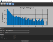
• Plot histograms of selected measurements, as shown below.

  

• Export results to a CSV file for additional analysis.

Creating Sparse Graphs

The result of creating a sparse graph is a model of connected areas in which the spheres and lines representing those areas and their connections can be examined in a 3D view, as shown below.

Sparse graph

The following measurements are available for sparse graphs.

Sparse graph measurements

	Description
Edge	The following can be applied as the edge measurement and edge LUT measurement. Euclidean Length… Is the Euclidean length of the line connecting two branches or a branch and end node. Note You can also import edge scalar values from a comma-separated values (*.csv extension) file (see ).
Vertex	By default, vertex measurements are not available for sparse graphs. However, you can map vertex scalar values from another object, such as a distance map, or import vertex scalar values from a comma-separated values (*.csv extension) file (see ). Other options include adding a vertex connectivities measurement or a constant vertex measurement (see Adding Constant Edge and Vertex Measurements).

How to Create a Sparse Graph

1. Create the required region of interest.

   For example, an ROI that describes a void or pore space.

2. Right-click the ROI in the Data Properties and Settings panel and then choose 3D Modeling > Create Sparse Graph in the pop-up menu.

   When skeletonization, labeling, and all other computations are complete, the graph appears in the Data Properties and Settings panel.

3. Select the graph in the Data Properties and Settings panel and then display it in a 3D view.
4. Adjust the graph settings, as required (see Graph Properties and Settings).

   Note You can also evaluate graphs with the Measurement Inspector (see Evaluating Graphs with the Measurement Inspector).

Creating Dense Graphs

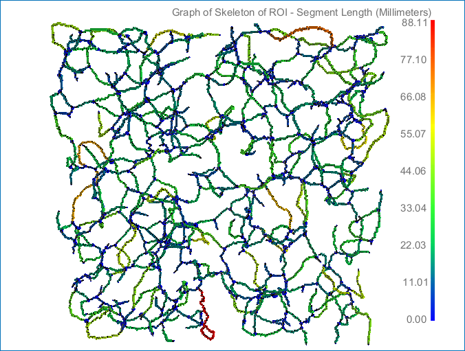
The result of creating a dense graph is a model of connected areas in which the spheres and lines representing those areas and their connections can be examined in a 3D view, as shown below. The measurements available for lines representing connected areas include tortuosity, length, and Euclidean length.

Dense graph

The following measurements are available for dense graphs.

Dense graph measurements

	Description
Edge	The following can be applied as the edge measurement and edge LUT measurement. Euclidean Length… Is the Euclidean length of the line connecting two branches or a branch and end node. Note You can also import edge scalar values from a comma-separated values (*.csv extension) file (see ).
Vertex	The following can be applied as the vertex radius measurement and vertex LUT measurement. Segment Tortuosity… Is a measure of the segment's tortuosity, which is calculated as Segment Length/Segment Euclidean Length. Segment Length… Is the actual length of the segment connecting two branches or connecting a branch with an end node. Segment Index… Is the index number, or identifier, assigned to each segment. Segment Euclidean Length… Is the Euclidean length of the segment connecting two branches or connecting a branch with an end node. Note You can map vertex scalar values from another object, such as a distance map, or import vertex scalar values from a comma-separated values (*.csv extension) file (see ). Other options include adding a vertex connectivities measurement or a constant vertex measurement (see Adding Constant Edge and Vertex Measurements).

For dense graphs, you can also plot graph tortuosity and throat-weight tortuosity (see Plotting Graph Tortuosity).

How to Create a Dense Graph

1. Create the required region of interest.

   For example, an ROI that describes a void or pore space.

2. Right-click the ROI in the Data Properties and Settings panel and then choose 3D Modeling > Create Dense Graph in the pop-up menu.

   When skeletonization, labeling, and all other computations are complete, the graph appears in the Data Properties and Settings panel.

3. Select the graph in the Data Properties and Settings panel and then display it in a 3D view.
4. Adjust the graph settings, as required (see Graph Properties and Settings).

   Note You can also evaluate graphs with the Measurement Inspector (see Evaluating Graphs with the Measurement Inspector).